28 Jul 2017, 13:14

Learning / R / Open Data

What are we about to do?

Learn the most important idioms for data munging in R
Apply them to an open data example
By the end, I hope you can use these skills to repeat this process with data you find

What Data Are We Using?

Kentucky Department of Education College and Career Readiness Data
Easily Found on their website

Step 1: Load Up Tidyverse and Read In Data

library(tidyverse)

ccr_data <- read_csv('./EDA_Munging_data/1516.csv')

glimpse(ccr_data)

## Observations: 6,902
## Variables: 25
## $ SCH_YEAR                   <int> 20152016, 20152016, 20152016, 20152...
## $ CNTYNO                     <chr> "001", "001", "001", "001", "001", ...
## $ CNTYNAME                   <chr> "ADAIR", "ADAIR", "ADAIR", "ADAIR",...
## $ DIST_NUMBER                <chr> "001", "001", "001", "001", "001", ...
## $ DIST_NAME                  <chr> "Adair County", "Adair County", "Ad...
## $ SCH_NUMBER                 <chr> "010", "010", "010", "010", "010", ...
## $ SCH_NAME                   <chr> "Adair County High School", "Adair ...
## $ SCH_CD                     <chr> "001010", "001010", "001010", "0010...
## $ SCH_TYPE                   <chr> "A1", "A1", "A1", "A1", "A1", "A1",...
## $ STATE_SCH_ID               <chr> "001001010", "001001010", "00100101...
## $ NCESID                     <dbl> 2.10003e+11, 2.10003e+11, 2.10003e+...
## $ CATEGORY                   <chr> "Accountability", "Accountability",...
## $ TEST_TYPE                  <chr> "CCR", "CCR", "CCR", "CCR", "CCR", ...
## $ DISAGG_ORDER               <int> 0, 1, 2, 3, 4, 5, 6, 7, 8, 9, 10, 1...
## $ DISAGG_LABEL               <chr> "All Students", "Male", "Female", "...
## $ NBR_GRADUATES_WITH_DIPLOMA <chr> "196", "106", "90", "180", "5*", "8...
## $ COLLEGE_READY              <int> 112, 54, 58, 106, NA, NA, NA, NA, N...
## $ CAREER_READY_ACADEMIC      <int> 134, 70, 64, 124, NA, NA, NA, NA, N...
## $ CAREER_READY_TECHNICAL     <int> 79, 44, 35, 77, NA, NA, NA, NA, NA,...
## $ CAREER_READY_TOTAL         <int> 72, 40, 32, 72, NA, NA, NA, NA, NA,...
## $ NBR_CCR_REGULAR            <int> 131, 65, 66, 125, NA, NA, NA, NA, N...
## $ PCT_CCR_NO_BONUS           <dbl> 66.8, 61.3, 73.3, 69.4, NA, NA, NA,...
## $ PCT_CCR_WITH_BONUS         <dbl> 80.9, 75.5, 87.2, 84.4, NA, NA, NA,...
## $ COOP                       <chr> "GRREC", "GRREC", "GRREC", "GRREC",...
## $ COOP_CODE                  <int> 902, 902, 902, 902, 902, 902, 902, ...

What do we have here?
- Is this data Wide or Narrow? (or both?!?!?!)
  - Wide data has columns for each variable
  - Narrow data typically has a “variable” column and a “value” column and each variable is repeated multiple times.
  - R very much prefers narrow data
- What columns seem important?
  - Does this data have multiple columns that represent the same value?
  - Are there columns that don’t contain useful information?
  - Consider your purpose for looking at the data, what story seems interesting and relevant?

# Look at data
glimpse(ccr_data)

## Observations: 6,902
## Variables: 25
## $ SCH_YEAR                   <int> 20152016, 20152016, 20152016, 20152...
## $ CNTYNO                     <chr> "001", "001", "001", "001", "001", ...
## $ CNTYNAME                   <chr> "ADAIR", "ADAIR", "ADAIR", "ADAIR",...
## $ DIST_NUMBER                <chr> "001", "001", "001", "001", "001", ...
## $ DIST_NAME                  <chr> "Adair County", "Adair County", "Ad...
## $ SCH_NUMBER                 <chr> "010", "010", "010", "010", "010", ...
## $ SCH_NAME                   <chr> "Adair County High School", "Adair ...
## $ SCH_CD                     <chr> "001010", "001010", "001010", "0010...
## $ SCH_TYPE                   <chr> "A1", "A1", "A1", "A1", "A1", "A1",...
## $ STATE_SCH_ID               <chr> "001001010", "001001010", "00100101...
## $ NCESID                     <dbl> 2.10003e+11, 2.10003e+11, 2.10003e+...
## $ CATEGORY                   <chr> "Accountability", "Accountability",...
## $ TEST_TYPE                  <chr> "CCR", "CCR", "CCR", "CCR", "CCR", ...
## $ DISAGG_ORDER               <int> 0, 1, 2, 3, 4, 5, 6, 7, 8, 9, 10, 1...
## $ DISAGG_LABEL               <chr> "All Students", "Male", "Female", "...
## $ NBR_GRADUATES_WITH_DIPLOMA <chr> "196", "106", "90", "180", "5*", "8...
## $ COLLEGE_READY              <int> 112, 54, 58, 106, NA, NA, NA, NA, N...
## $ CAREER_READY_ACADEMIC      <int> 134, 70, 64, 124, NA, NA, NA, NA, N...
## $ CAREER_READY_TECHNICAL     <int> 79, 44, 35, 77, NA, NA, NA, NA, NA,...
## $ CAREER_READY_TOTAL         <int> 72, 40, 32, 72, NA, NA, NA, NA, NA,...
## $ NBR_CCR_REGULAR            <int> 131, 65, 66, 125, NA, NA, NA, NA, N...
## $ PCT_CCR_NO_BONUS           <dbl> 66.8, 61.3, 73.3, 69.4, NA, NA, NA,...
## $ PCT_CCR_WITH_BONUS         <dbl> 80.9, 75.5, 87.2, 84.4, NA, NA, NA,...
## $ COOP                       <chr> "GRREC", "GRREC", "GRREC", "GRREC",...
## $ COOP_CODE                  <int> 902, 902, 902, 902, 902, 902, 902, ...

# Unique values in each column
map(ccr_data %>% filter(DIST_NAME == 'Jefferson County'), function(i) length(unique(i)))

## $SCH_YEAR
## [1] 1
## 
## $CNTYNO
## [1] 1
## 
## $CNTYNAME
## [1] 1
## 
## $DIST_NUMBER
## [1] 1
## 
## $DIST_NAME
## [1] 1
## 
## $SCH_NUMBER
## [1] 22
## 
## $SCH_NAME
## [1] 22
## 
## $SCH_CD
## [1] 22
## 
## $SCH_TYPE
## [1] 2
## 
## $STATE_SCH_ID
## [1] 22
## 
## $NCESID
## [1] 22
## 
## $CATEGORY
## [1] 1
## 
## $TEST_TYPE
## [1] 1
## 
## $DISAGG_ORDER
## [1] 17
## 
## $DISAGG_LABEL
## [1] 17
## 
## $NBR_GRADUATES_WITH_DIPLOMA
## [1] 149
## 
## $COLLEGE_READY
## [1] 116
## 
## $CAREER_READY_ACADEMIC
## [1] 61
## 
## $CAREER_READY_TECHNICAL
## [1] 81
## 
## $CAREER_READY_TOTAL
## [1] 48
## 
## $NBR_CCR_REGULAR
## [1] 122
## 
## $PCT_CCR_NO_BONUS
## [1] 169
## 
## $PCT_CCR_WITH_BONUS
## [1] 168
## 
## $COOP
## [1] 1
## 
## $COOP_CODE
## [1] 1

# Don't forget the glossary!
# http://applications.education.ky.gov/SRC/Glossary.aspx

## Looking at the data by county, selecting just the columns we are interested in

ccr_data_s <- ccr_data %>% 
  filter(DIST_NAME == 'Jefferson County') %>% 
  select(SCH_YEAR, SCH_NAME, DISAGG_LABEL, NBR_GRADUATES_WITH_DIPLOMA, NBR_CCR_REGULAR, PCT_CCR_NO_BONUS)

glimpse(ccr_data_s)

## Observations: 374
## Variables: 6
## $ SCH_YEAR                   <int> 20152016, 20152016, 20152016, 20152...
## $ SCH_NAME                   <chr> "Atherton High School", "Atherton H...
## $ DISAGG_LABEL               <chr> "All Students", "Male", "Female", "...
## $ NBR_GRADUATES_WITH_DIPLOMA <chr> "264", "114", "150", "175", "59", "...
## $ NBR_CCR_REGULAR            <int> 209, 82, 127, 150, 32, 13, NA, NA, ...
## $ PCT_CCR_NO_BONUS           <dbl> 79.2, 71.9, 84.7, 85.7, 54.2, 81.3,...

WTF JUST HAPPENED

The first thing we did was to load the tidyverse. This gives use access to many of the most powerful data analysis packages.
- dplyr is a “grammar of data manipulation” and was written by Hadley Wickham.
  - Four idioms in dplyr are the most important: select, filter, mutate, and summarize
- We’ve technically already used both readr with read_csv and also tibble.
filter - a subsetting function. Takes column names and equivilencies as arguments.
select - a function for picking columns.
- select has a lot of helper functions, and negative values can be used.
%>% - the pipe. Linux people can guess what this means.
- Originally from the magrittr package. I have no idea what magrittr was supposed to do, but it gave use the pipe.
- When you see this, the data on the LHS becomes the first argument to the function on the RHS
- Once you get the hang of %>%, your life will change for the better
- A massive amount of R base functions have been rewritten so the data is the first argument.
BONUS map is from purrr. It is a unique way to do iteration in R. If we have time, I’ll talk about it at the end.

Okay, So What Now?

Are there any type issues?
Let’s explore our narrow columns to see if there are any inconsistencies.

ccr_data_s %>% glimpse()

## Observations: 374
## Variables: 6
## $ SCH_YEAR                   <int> 20152016, 20152016, 20152016, 20152...
## $ SCH_NAME                   <chr> "Atherton High School", "Atherton H...
## $ DISAGG_LABEL               <chr> "All Students", "Male", "Female", "...
## $ NBR_GRADUATES_WITH_DIPLOMA <chr> "264", "114", "150", "175", "59", "...
## $ NBR_CCR_REGULAR            <int> 209, 82, 127, 150, 32, 13, NA, NA, ...
## $ PCT_CCR_NO_BONUS           <dbl> 79.2, 71.9, 84.7, 85.7, 54.2, 81.3,...

ccr_data_s$SCH_NAME %>% unique() %>% sort()

##  [1] "---District Total---"           "Atherton High School"          
##  [3] "Ballard High"                   "Brown School"                  
##  [5] "Butler Traditional High School" "Central High School"           
##  [7] "Doss High"                      "duPont Manual High"            
##  [9] "Eastern High"                   "Fairdale High School"          
## [11] "Fern Creek High School"         "Iroquois High"                 
## [13] "Jeffersontown High School"      "Louisville Male High School"   
## [15] "Moore Traditional School"       "Pleasure Ridge Park High"      
## [17] "Seneca High"                    "Southern High School"          
## [19] "The Academy @ Shawnee"          "Valley High School"            
## [21] "Waggener High School"           "Western High School"

# Fix up some columns!

library(stringr)
ccr_data_t <- ccr_data_s %>% 
  mutate(
    SCH_NAME = str_replace_all(SCH_NAME, '[[:punct:]]','') %>% trimws(),
    SCH_YEAR = 2016,
    NBR_GRADUATES_WITH_DIPLOMA = str_replace_all(NBR_GRADUATES_WITH_DIPLOMA, '[[:punct:]]','') %>% as.numeric(),
    NBR_CCR_REGULAR = str_replace_all(NBR_CCR_REGULAR, '[[:punct:]]','') %>% as.numeric()
  )

glimpse(ccr_data_t)

## Observations: 374
## Variables: 6
## $ SCH_YEAR                   <dbl> 2016, 2016, 2016, 2016, 2016, 2016,...
## $ SCH_NAME                   <chr> "Atherton High School", "Atherton H...
## $ DISAGG_LABEL               <chr> "All Students", "Male", "Female", "...
## $ NBR_GRADUATES_WITH_DIPLOMA <dbl> 264, 114, 150, 175, 59, 16, 9, 1, N...
## $ NBR_CCR_REGULAR            <dbl> 209, 82, 127, 150, 32, 13, NA, NA, ...
## $ PCT_CCR_NO_BONUS           <dbl> 79.2, 71.9, 84.7, 85.7, 54.2, 81.3,...

Mutate and `stringr`

Of all the dplyr functions, mutate is my favorite
mutate takes a column, applies a transformation to it, and either saves it back into the old column or creates a new column.
- Great for using iterators like the apply family or the purrr::map family.
stringr is another tidyverse package, but it needs to be loaded separately.
- There are a lot of basic string functions built into base R, but they don’t have the data as the first argument, and can’t be used with the %>%.
- It’s PROBABLY a good idea to learn about the base R functions, but IMO, learning stringr is better.
- There are other, more powerful string function in stringr not available in base R.
We also used as.numeric() which is a casting function. BE CAREFUL with these.
- If we hadn’t pulled out the extra punctuation first, it would have cast the non-numeric data to NA.

Narrow It Down

We’ve still got Wide data. Let’s narrow it up!

ccr_data_n <- ccr_data_t %>% 
    gather(key = Level, value = value, NBR_GRADUATES_WITH_DIPLOMA,NBR_CCR_REGULAR,PCT_CCR_NO_BONUS)

glimpse(ccr_data_n)

## Observations: 1,122
## Variables: 5
## $ SCH_YEAR     <dbl> 2016, 2016, 2016, 2016, 2016, 2016, 2016, 2016, 2...
## $ SCH_NAME     <chr> "Atherton High School", "Atherton High School", "...
## $ DISAGG_LABEL <chr> "All Students", "Male", "Female", "White (Non-His...
## $ Level        <chr> "NBR_GRADUATES_WITH_DIPLOMA", "NBR_GRADUATES_WITH...
## $ value        <dbl> 264, 114, 150, 175, 59, 16, 9, 1, NA, 4, NA, 5, 1...

`Gather`, or, the most confusing thing in the world.

Back in the day, many people used a package named reshape2
- Many people still use it. The best part was reshape2::melt, which made data narrow.
tidyr::gather is, in my mind, a better solution. It’s part of the tidyverse and make things more explicit.
- gather takes a key and a value, which are NEW columns that will be created.
- Then, you pass it the columns you want to gather and those get placed into the key column
  - I told you this was confusing.
- There is a partner to gather, spread, which takes narrow data and makes it wide.

Next Up, Listen for Tips!

Kris Stevens gave me this data, and told me that many of the “District Total” figures weren’t correct.
Let’s fix them up!

ccr_data_n %>% 
    filter(Level == 'NBR_GRADUATES_WITH_DIPLOMA') %>% 
    group_by(DISAGG_LABEL) %>% 
    summarize('NBR_GRADUATES_WITH_DIPLOMA' = sum(value, na.rm = T)) %>% 
    left_join(
      ccr_data_n %>% 
        filter(Level == 'NBR_CCR_REGULAR') %>% 
        group_by(DISAGG_LABEL) %>% 
        summarize('NBR_CCR_REGULAR' = sum(value, na.rm = T))
    ) %>% 
    mutate(PCT_CCR_NO_BONUS = round(100 * (NBR_CCR_REGULAR / NBR_GRADUATES_WITH_DIPLOMA ))) %>% 
    gather(key = Level, value = value, NBR_GRADUATES_WITH_DIPLOMA,NBR_CCR_REGULAR,PCT_CCR_NO_BONUS) %>% 
    mutate(SCH_YEAR = 2016,
           SCH_NAME = 'District Total') %>% 
    bind_rows(ccr_data_n) %>% View()

Woof, that code is ugly. Is there a better way?

aggregate_level <- function(df, col_head){
  df %>% 
    filter(Level == col_head) %>% 
    group_by(DISAGG_LABEL) %>% 
    summarize(new_col = sum(value, na.rm = T)) %>% 
    rename_(.dots = setNames('new_col', eval(col_head)))
}

ccr_tidy <- aggregate_level(ccr_data_n, 'NBR_GRADUATES_WITH_DIPLOMA') %>% 
  left_join(aggregate_level(ccr_data_n, 'NBR_CCR_REGULAR')) %>% 
    mutate(PCT_CCR_NO_BONUS = round(100 * (NBR_CCR_REGULAR / NBR_GRADUATES_WITH_DIPLOMA ))) %>% 
    gather(key = Level, value = value, NBR_GRADUATES_WITH_DIPLOMA,NBR_CCR_REGULAR,PCT_CCR_NO_BONUS) %>% 
    mutate(SCH_YEAR = 2016,
           SCH_NAME = 'District Total') %>% 
    bind_rows(ccr_data_n)

`group_by`, `summarize`, joins, binds, NSE, and functional programming

WHAT A LIST
If you’ve used SQL, you probably understand group_by.
- When you group a column and then run an aggregation function, it aggregates PER GROUP.
summarize is one of those aggregation functions.
- summarize is kind of like mutate, but instead of creating a new column of the same length as the df, it summarizes the data.
- There are places where summarize is useful without group_by, but not many.
- The way we used summarize above, we got a number representing the sum of value by each DISAGG_LABEL .
  - We could have switched the group_by to SCH_NAME and it would have given us the sum of value by each school.
- It’s technically summarise, but this is America, dammit.
Joins are also something SQL users will be familiar with.
- Types: left_join, inner_join, right_join, full_join, semi_join, and anti_join.
- All types take two data frames, and typically a by argument, and sometimes a suffix argument.
  - by takes a vector that looks like c('lhs' = 'rhs')
  - If there are column names in common with LHS and RHS, the default suffix is ‘.x’ and ‘.y’, but you can override those.
- We are using left_join:
  - “return all rows from x where there are matching values in y, and all columns from x and y. If there are multiple matches between x and y, all combination of the matches are returned.”
- The R documentation for joins is good if you aren’t clear about which of these. anti_join and semi_join are rare but cool.
Binds are way to bind together data frames. They stack on top of each other.
- bind_rows and bind_cols are the dplyr way to do things.
- rbind and cbind are base R.
- As usualy, the tidyverse way is safer and more powerful.
Non-standard evaluation
- If you’ve got keen eyes, you’ve noticed that the arguments to the dplyr functions are never strings – they are bare and unquoted.
- This form of evaluation is called “standard evaluation”, and it’s not great for programming. (Fine for analysis though).
- “Non-Standard Evaluation” is also present in dplyr. It’s all the functions with an underscore after them. For example rename_ (rename is another way to do select)
  - Probably don’t worry about knowing how to do this, but know it’s there.
Functional Programming
- This is the heart of R – building functions you can call later.
- Everything we’ve “called” so far is technically a function. You can build your own!
- function(x,y){} would create a function that you could call with two inputs.
- Most of the functions I write are anonymous, but not always!

OKAY SO WHAT NEXT

We’ve been working with one csv’s worth of data so far, but the BoE makes several years available. Let’s combine them!
To do that, we will put all the code we’ve made so far into a function, and then bind all the data together using that function.

tidy_ccr <- function(df, county){
  tidy_df <- df %>% 
    filter(DIST_NAME == county) %>% 
    select(SCH_YEAR, SCH_NAME, DISAGG_LABEL, NBR_GRADUATES_WITH_DIPLOMA, NBR_CCR_REGULAR, PCT_CCR_NO_BONUS) %>% 
    mutate(      # First Change
      SCH_YEAR = case_when(SCH_YEAR == 20152016 ~ 2016L,
          SCH_YEAR == 20142015 ~ 2015L,
          SCH_YEAR == 20132014 ~ 2014L,
          SCH_YEAR == 20122013 ~ 2013L,
          SCH_YEAR == 20112012 ~ 2012L
        ) %>% ordered(),
      SCH_NAME = str_replace_all(SCH_NAME, '[[:punct:]]','') %>% trimws(),
      NBR_GRADUATES_WITH_DIPLOMA = str_replace_all(NBR_GRADUATES_WITH_DIPLOMA, '[[:punct:]]','') %>% as.numeric(),
      NBR_CCR_REGULAR = str_replace_all(NBR_CCR_REGULAR, '[[:punct:]]','') %>% as.numeric()
    ) %>% 
    gather(key = Level, value = value, NBR_GRADUATES_WITH_DIPLOMA,NBR_CCR_REGULAR,PCT_CCR_NO_BONUS)
  
  aggregate_level(tidy_df, 'NBR_GRADUATES_WITH_DIPLOMA') %>% 
    left_join(aggregate_level(tidy_df, 'NBR_CCR_REGULAR')) %>% 
    mutate(PCT_CCR_NO_BONUS = round(100 * (NBR_CCR_REGULAR / NBR_GRADUATES_WITH_DIPLOMA ))) %>% 
    gather(key = Level, value = value, NBR_GRADUATES_WITH_DIPLOMA,NBR_CCR_REGULAR,PCT_CCR_NO_BONUS) %>% 
    mutate(SCH_YEAR = tidy_df$SCH_YEAR[1],
           SCH_NAME = 'District Total') %>% 
    bind_rows(tidy_df)
}

bind_data <- function(county){
  bind_rows(
    read_csv('./EDA_Munging_data/1516.csv') %>% tidy_ccr(county),
    read_csv('./EDA_Munging_data/1415.csv') %>% tidy_ccr(county),
    read_csv('./EDA_Munging_data/1314.csv') %>% tidy_ccr(county),
    read_csv('./EDA_Munging_data/1213.csv') %>% tidy_ccr(county),
    read_csv('./EDA_Munging_data/1112.csv') %>% tidy_ccr(county)
  )
}

jefferson_data <- bind_data('Jefferson County')

Now You Get It!

You get it, right?
- What does the bind_data function do? Can you explain it?
I also made a change to the SCH_YEAR column, so that it work correctly.
- case_when is a sexy way to do ifelse.
- I also used another map function.
Okay, so let’s take a look to make sure things aren’t too weird.

glimpse(jefferson_data)

## Observations: 5,865
## Variables: 5
## $ DISAGG_LABEL <chr> "African American", "All Students", "American Ind...
## $ Level        <chr> "NBR_GRADUATES_WITH_DIPLOMA", "NBR_GRADUATES_WITH...
## $ value        <dbl> 4135, 11958, 12, 493, 112, 333, 445, 401, 6276, 6...
## $ SCH_YEAR     <chr> "2016", "2016", "2016", "2016", "2016", "2016", "...
## $ SCH_NAME     <chr> "District Total", "District Total", "District Tot...

jefferson_data$DISAGG_LABEL %>% unique()

##  [1] "African American"                             
##  [2] "All Students"                                 
##  [3] "American Indian or Alaska Native"             
##  [4] "Asian"                                        
##  [5] "Disability-Alternate Only"                    
##  [6] "Disability-With IEP (not including Alternate)"
##  [7] "Disability-With IEP (Total)"                  
##  [8] "English Learners"                             
##  [9] "Female"                                       
## [10] "Free/Reduced-Price Meals"                     
## [11] "Gap Group (non-duplicated)"                   
## [12] "Hispanic"                                     
## [13] "Male"                                         
## [14] "Migrant"                                      
## [15] "Native Hawaiian or Other Pacific Islander"    
## [16] "Two or more races"                            
## [17] "White (Non-Hispanic)"                         
## [18] "Limited English Proficiency"

jefferson_data$SCH_NAME %>% unique()

##  [1] "District Total"                 "Atherton High School"          
##  [3] "Ballard High"                   "Brown School"                  
##  [5] "Butler Traditional High School" "Central High School"           
##  [7] "Doss High"                      "Eastern High"                  
##  [9] "Fairdale High School"           "Fern Creek High School"        
## [11] "Iroquois High"                  "Jeffersontown High School"     
## [13] "Louisville Male High School"    "Moore Traditional School"      
## [15] "Pleasure Ridge Park High"       "Seneca High"                   
## [17] "Southern High School"           "The Academy  Shawnee"          
## [19] "Valley High School"             "Waggener High School"          
## [21] "Western High School"            "duPont Manual High"            
## [23] "Dupont Manual High"             "Fern Creek Traditional High"   
## [25] "Fairdale High School MCA"

tidy_ccr <- function(df, county){
  tidy_df <- df %>% 
    filter(DIST_NAME == county) %>% 
    select(SCH_YEAR, SCH_NAME, DISAGG_LABEL, NBR_GRADUATES_WITH_DIPLOMA, NBR_CCR_REGULAR, PCT_CCR_NO_BONUS) %>% 
    mutate(
      SCH_YEAR = case_when(
          SCH_YEAR == 20152016 ~ 2016L,
          SCH_YEAR == 20142015 ~ 2015L,
          SCH_YEAR == 20132014 ~ 2014L,
          SCH_YEAR == 20122013 ~ 2013L,
          SCH_YEAR == 20112012 ~ 2012L
        ) %>% ordered(),
      SCH_NAME = map_chr(SCH_NAME, function(i){
        if(i == 'Dupont Manual High') 'duPont Manual High'
        else if(i == 'Fern Creek Traditional High') 'Fern Creek High School'
        else if(i == 'Fairdale High School MCA') 'Fairdale High School'
        else str_replace_all(i, '[[:punct:]]','') %>% trimws()
      }),
      NBR_GRADUATES_WITH_DIPLOMA = str_replace_all(NBR_GRADUATES_WITH_DIPLOMA, '[[:punct:]]','') %>% as.numeric(),
      NBR_CCR_REGULAR = str_replace_all(NBR_CCR_REGULAR, '[[:punct:]]','') %>% as.numeric()
    ) %>% 
    gather(key = Level, value = value, NBR_GRADUATES_WITH_DIPLOMA,NBR_CCR_REGULAR,PCT_CCR_NO_BONUS)
  
  aggregate_level(tidy_df, 'NBR_GRADUATES_WITH_DIPLOMA') %>% 
    left_join(aggregate_level(tidy_df, 'NBR_CCR_REGULAR')) %>% 
    mutate(PCT_CCR_NO_BONUS = round(100 * (NBR_CCR_REGULAR / NBR_GRADUATES_WITH_DIPLOMA ))) %>% 
    gather(key = Level, value = value, NBR_GRADUATES_WITH_DIPLOMA,NBR_CCR_REGULAR,PCT_CCR_NO_BONUS) %>% 
    mutate(SCH_YEAR = tidy_df$SCH_YEAR[1],
           SCH_NAME = 'District Total') %>% 
    bind_rows(tidy_df)
}

jefferson_data <- bind_data('Jefferson County')

Fixing the Weirdness

The SCH_NAME field was not consistent across the data, so we fixed it.
- We used an iterator, which is a little more advaced than we are going today (probably)

NOW WE’VE GOT TIDY DATA!!!!

Let’s do some basic visualizations!

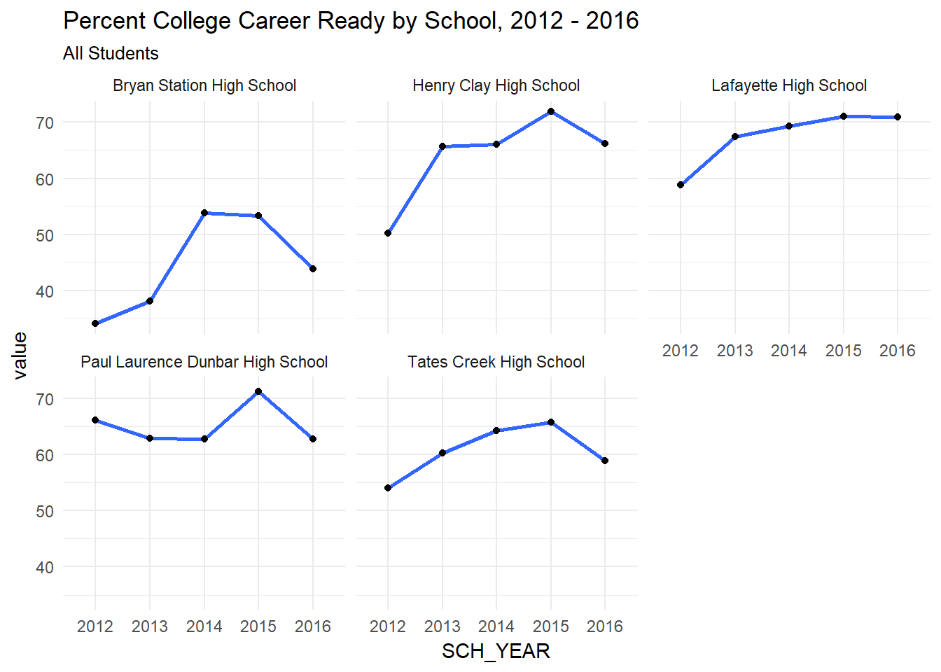
facet_ccr <- function(df, lev){
  ggplot(df %>% 
         filter(SCH_NAME != 'District Total',
                Level == 'PCT_CCR_NO_BONUS', 
                DISAGG_LABEL == lev), 
       aes(x = SCH_YEAR, y = value, group = 1)) + 
  geom_smooth() +
  geom_point() +
  ggtitle('Percent College Career Ready by School, 2012 - 2016',
          subtitle = lev) +
  facet_wrap(~SCH_NAME) +
  theme_minimal()
}

j<- bind_data('Jefferson County')
f <- bind_data('Fayette County')

facet_ccr(j, 'All Students')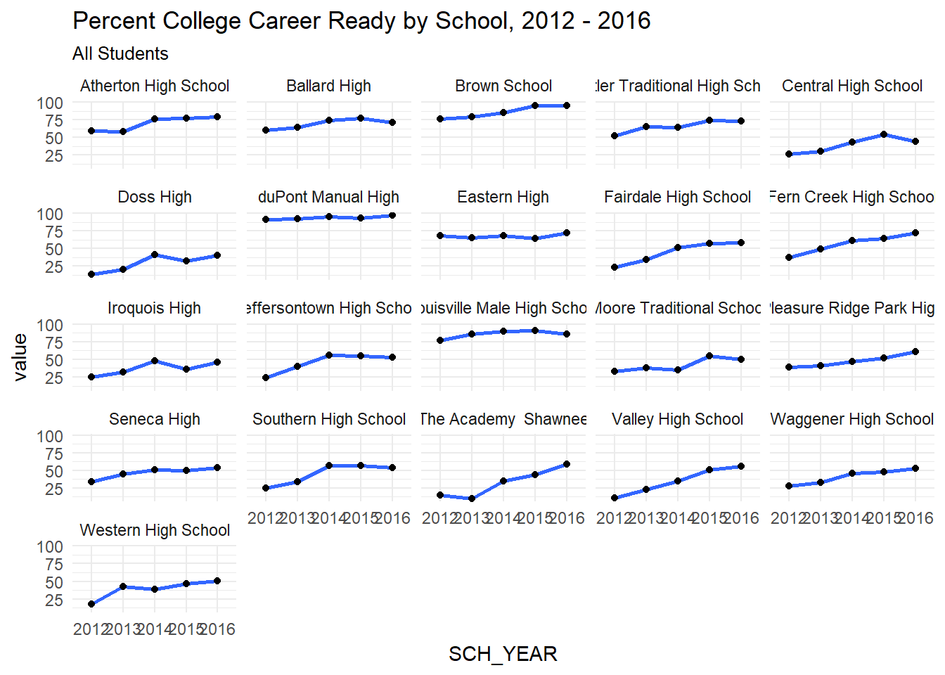

facet_ccr(f, 'All Students')

EDA and Basic Data Munging with Public Data

What are we about to do?

What Data Are We Using?

Step 1: Load Up Tidyverse and Read In Data

WTF JUST HAPPENED

Okay, So What Now?

Mutate and stringr

Narrow It Down

Gather, or, the most confusing thing in the world.

Next Up, Listen for Tips!

Woof, that code is ugly. Is there a better way?

group_by, summarize, joins, binds, NSE, and functional programming

OKAY SO WHAT NEXT

Now You Get It!

Fixing the Weirdness

NOW WE’VE GOT TIDY DATA!!!!

Mutate and `stringr`

`Gather`, or, the most confusing thing in the world.

`group_by`, `summarize`, joins, binds, NSE, and functional programming